Logistic Regression in Machine Learning: The Ultimate Guide

Welcome to this comprehensive tutorial on logistic regression in machine learning. If you've been working with linear models and now want to predict categories instead of continuous numbers—perhaps predicting if an email is a "Spam" or "Not Spam"—you are in the right place. Have you been searching for "logistic regression what is"? Let's dive deep into its core mechanics, profound theory, and practical implementation.

1. Logistic Regression Meaning & What It Is

Despite having the word "regression" in its name, logistic regression machine learning is predominantly used as a supervised classification algorithm. The logistic regression meaning fundamentally revolves around estimating the mathematical probability that an instance belongs to a particular class. If the estimated probability is greater than a set threshold (usually 50%), the model predicts that the instance belongs to that target class (called the positive class, labeled "1"). If the probability is less than 50%, it predicts it does not belong (the negative class, labeled "0").

This structural behavior makes it an incredibly powerful binary classifier. It is the gold standard for logistic regression analysis in fields that require definitive binary outcomes (True/False, Yes/No, Win/Loss, Healthy/Sick).

2. Linear Regression vs Logistic Regression Machine Learning

One of the most frequently asked questions by beginners is how this differs from linear regression. Linear regression tries to predict a continuous numerical value (like predicting a house price of $450,000 or a temperature of 72°F) by fitting a straight line. However, if you apply a straight line to binary classification, the line will continue indefinitely into negative and positive numbers. A probability of -200% or +400% makes absolutely no mathematical sense!

Conversely, logistic regression in machine learning squeezes the output of that linear equation strictly between 0 and 1, ensuring the output is always a valid probability.

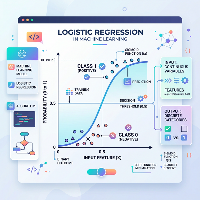
3. The S-Shaped Logistic Regression Graph

To keep the predicted outputs strictly bounded between 0 and 1, the model utilizes the mathematical Sigmoid function. When you plot these probabilities on a chart, the logistic regression graph forms a very distinctive S-shaped curve (called an ogive).

Unlike linear regression which draws a straight line that spans to infinity, the Sigmoid curve beautifully categorizes your feature data, plateauing at 0 on the bottom and 1 at the top, making a clear boundary line where predictions tilt from one category to another at the 0.5 center point.

4. The Logistic Regression Formula Explained

At its heart, logistic regression computes a weighted sum of the input features (exactly like linear regression), but instead of outputting the sum directly, it passes that result through the logistic (sigmoid) function. The core logistic regression formula is:

P(y=1) = 1 / (1 + e^{-(β₀
+ β₁X)})

Where:

P(y=1): The calculated probability that the outcome is 1 (the positive class).
e: Euler's number (the base of the natural logarithm, approximately 2.718).
β₀ & β₁X: The standard linear equation representing biases and weights multiplied by your feature inputs (X).

5. The Logistic Regression Cost Function & Maximum Likelihood

How does the model actually learn the best values for the weights (β)? In linear regression, we simply use the Mean Squared Error (MSE) to find the line of best fit. However, if you insert the non-linear Sigmoid formula into the MSE equation, it results in a non-convex function that resembles a roller coaster full of false local minimums. Gradient Descent would get stuck!

Because of this, the logistic regression cost function uses a principle called Maximum Likelihood Estimation (MLE), mathematically represented as Log Loss (or Binary Cross-Entropy).

Log Loss heavily penalizes models that are "confident but wrong." If a poorly tuned model predicts a probability of 0.999 for a class that actually turns out to be 0, the cost function rockets up exponentially almost to infinity. Optimization algorithms like Gradient Descent minimize this cost function during training, smoothing out the curve.

6. Key Logistic Regression Assumptions

Before you blindly feed data into an algorithm, you must ensure your dataset conforms to these core logistic regression assumptions to ensure accurate logistic regression analysis:

Binary Outcome: The target dependent variable must be strictly binary (although variants like Multinomial Logistic Regression exist for multi-class problems).
Independence of Observations: Observations should not come from repeated measurements (like time-series data on the same patient).
No Multicollinearity: The independent predictor variables should not be highly correlated with each other. A correlation matrix is typically used to drop redundant columns.
Linearity of Log-Odds: It strictly requires a linear relationship between features and the "logit" (log-odds) of the outcome.
Lack of Extreme Outliers: The model can be skewed by severe outliers present in continuous predictive features.

7. Practical Logistic Regression Example Using Python

Theory is fantastic, but we are developers. Let's delve into a practical logistic regression example! If you search "logistic regression sklearn", you will find that the Python scikit-learn library makes it remarkably simple to implement binary classification with just a few lines of code.

Below is a standardized logistic regression sklearn python implementation. In this scenario, we use dummy medical data tracking the number of "Hours Slept" to predict if a student "Passed" (y=1) or "Failed" (y=0) their final examination.

# 1. Import necessary components
import numpy as np
from sklearn.model_selection import train_test_split
from sklearn.linear_model import LogisticRegression
from sklearn.metrics import accuracy_score, confusion_matrix, classification_report

# 2. Dummy Data: Hours slept (X) predicting if a student passed exam (y=1) or failed (y=0)
X = np.array([2, 3, 4, 5, 6, 7, 8, 9, 10, 11]).reshape(-1, 1)
y = np.array([0, 0, 0, 0, 1, 1, 1, 1, 1, 1])

# 3. Split the dataset into Training and Testing sequences
X_train, X_test, y_train, y_test = train_test_split(X, y, test_size=0.2, random_state=42)

# 4. Initialize the Logistic Regression model
clf = LogisticRegression()

# 5. Train (fit) the model
clf.fit(X_train, y_train)

# 6. Make probability predictions against the testing data
predictions = clf.predict(X_test)
probabilities = clf.predict_proba(X_test)

# 7. Evaluate the health and success metrics of the classification
accuracy = accuracy_score(y_test, predictions)
print(f"Model Accuracy: {accuracy * 100}%")

print("\nConfusion Matrix:")
print(confusion_matrix(y_test, predictions))

print("\nProbabilities of [Class 0 vs Class 1]:")
print(np.round(probabilities, 2))

Conclusion

Understanding logistic regression in machine learning acts as a crucial stepping-stone to the more complex domains of deep learning. In fact, an isolated artificial neuron (the perceptron) inside a deep Neural Network is heavily structured around the exact mathematical principles of a logistic regressor using a sigmoid activation function.

Whether you're attempting to predict customer churn, diagnose malignant medical imagery, or filter spam messages out of an inbox, mastering the assumptions and cost functions of this elegant algorithm is mandatory for any competent data scientist.

Frequently Asked Questions (FAQs)

Why is it mathematically called "Regression" if it primarily solves "Classification" problems?

The confusing nomenclature is entirely historical. It uses the foundational mathematical calculations of standard linear regression as its base structure (calculating weighted sums) but wraps the final output in a Sigmoid activation curve to output a probability, mapping continuous numbers into discrete class categories. It technically "regresses" to the mean of a logit distribution.

What is a Confusion Matrix in Logistic Regression Analysis?

It is a visual performance measurement table used strictly for evaluating classification algorithms. It contrasts the model's predicted categories versus the actual ground-truth categories, neatly breaking them down into True Positives (Hits), True Negatives (Correct Rejections), False Positives (Type I Error), and False Negatives (Type II Error).

Can Logistic Regression handle more than two categories (e.g., Multi-Class Classification)?

Absolutely. While standard logistic regression represents a binary outcome, Multinomial Logistic Regression handles scenarios with 3 or more categories (e.g., predicting if a weather forecast is Rain, Sun, or Snow). Typically, this involves using the elegant Softmax function which calculates relative probabilities across classes that perfectly equal 1.0.