Machine Learning Linear Regression: A Comprehensive Guide

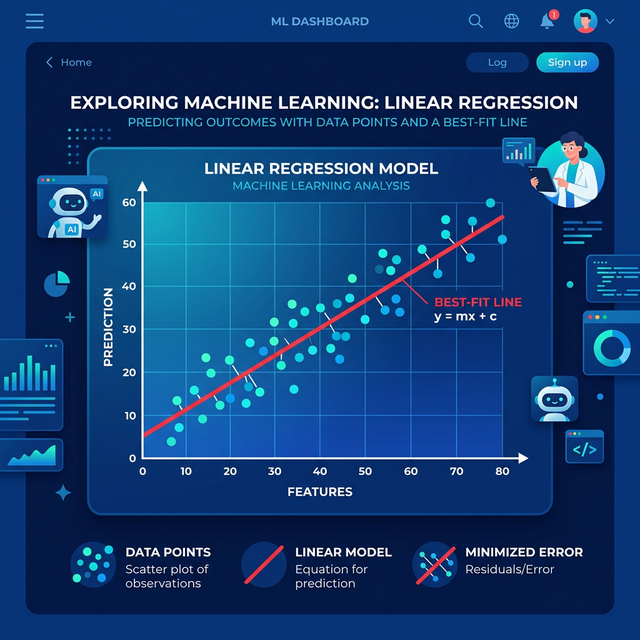
Welcome to this comprehensive and in-depth tutorial on one of the most foundational and popular algorithms in data science. If you are starting your journey into artificial intelligence and find yourself asking, what is linear regression in machine learning, you are in the right place. This guide will walk you through the core concepts, internal working mechanics, mathematical foundations, different variations, and a practical coding implementation in Python.

1. What is Linear Regression in Machine Learning?

At its core, linear regression is a supervised machine learning prediction algorithm used to understand the relationship between a continuous dependent variable (the target) and one or more independent variables (the predictors or features). By fitting a linear equation—often visualized as a straight line—to observed data, this algorithm attempts to forecast future outcomes based on given inputs.

In the expansive world of machine learning regression models, linear regression acts as the absolute baseline. Before engineers ever jump into complex neural networks or ensemble methods, they first try to fit a linear model. Its simplicity makes it easy to train, quick to deploy, and most importantly, highly interpretative. When a standard business stakeholder asks why a prediction was made, linear regression allows you to pinpoint exactly how much each feature contributed to the final output.

2. Types of Machine Learning Regression Algorithms & Models

When assessing machine learning regression algorithms, linear regression is typically categorized based on the number of predictor variables it uses. The primary types are:

Simple Linear Regression: Involves a single independent variable to predict a numerical dependent variable. For example, predicting a student's final exam score exclusively based on the number of hours they studied. The relationship maps naturally to a 2D plane (X and Y axis).
Multiple Linear Regression: Used when two or more independent variables are available to establish a relationship. A real-world scenario would be predicting a house's price based on its square footage, number of bedrooms, and distance from the city center. This maps to a multi-dimensional hyperspace.
Polynomial Regression: A subset configuration where the relationship between the independent variable x and the dependent variable y is modeled as an nth degree polynomial, dealing with non-linear relationships using linear techniques.

These machine learning regression models are widely used in a variety of fields, from real estate forecasting and sales projections to medical research and stock market analysis, primarily due to their robustness and interpretability.

3. The Linear Regression in Machine Learning Formula Explained

To truly understand how this model calculates its predictions, we must look at the underlying mathematics. The mathematical foundation powering this algorithm is elegant. The standard linear regression in machine learning formula for predicting a specific continuous value y in simple linear regression is given by:

Y = β₀ + β₁X + ε

Let's break down each component of this equation:

Y (Dependent Variable): The ultimate target variable we are trying to predict or estimate.
X (Independent Variable): The input predictor or feature we provide to the model.
β₀ (Y-Intercept): The expected mean value of Y when X is exactly zero. It comes in handy when defining where the regression line crosses the y-axis.
β₁ (Slope/Coefficient): Represents the magnitude of change in Y for a one-unit change in X. A positive slope indicates a positive correlation, while a negative slope indicates an inverse correlation.
ε (Error Term): This represents the residual error. It accounts for the variation in Y that cannot be perfectly explained by X. In a perfect world, all points fall natively on the best-fit line, but real-world data always contains noise.

4. How Does Linear Regression Actually Learn?

The goal of training our regression model is to find the perfect values for β₀ and β₁ that minimize the total error. The most common method used to accomplish this is called Ordinary Least Squares (OLS).

OLS works by calculating the vertical distance (called residuals) from every single data point to the proposed best-fit line, squaring those distances (to remove negative values and heavily penalize large errors), and summing them up. The algorithm then adjusts the line's position iteratively—often utilizing an optimization algorithm called Gradient Descent—until it discovers the line with the absolute minimum sum of squared errors.

5. Real-World Applications of Regression Problems

Before jumping into the practical implementation, let’s explore where this algorithm thrives in the business world:

Economics and Finance: Used extensively to predict economic growth, evaluate financial risk, and project future company revenues based on past performance metrics.
Real Estate: Utilizing features like location, square footage, age of the property, and nearest transit systems to accurately predict housing market valuation.
Marketing Effectiveness: Businesses calculate ROI by analyzing how advertising spend across different channels (TV, Radio, Social Media) impacts final product sales across time.

6. Linear Regression in Machine Learning Example & Code

The best way to solidify your understanding of these abstract concepts is to write the code yourself. Let's delve into a full linear regression in machine learning example. Below, we've provided some beautifully simple and effective linear regression in machine learning code using Python and the popular scikit-learn machine learning library.

This script generates synthetic relationships, splits the data, trains the model, and evaluates its accuracy.

Here is the Python implementation:

# 1. Import vital libraries for arrays, ML algorithms, and evaluation

import numpy as np

from sklearn.model_selection import train_test_split

from sklearn.linear_model import LinearRegression

from sklearn.metrics import mean_squared_error, r2_score



# 2. Provide the dataset (X = predictors, y = target to predict)

# Reshaping X allows scikit-learn to handle the 2D array structure

X = np.array([1, 2, 3, 4, 5, 6, 7, 8, 9, 10]).reshape(-1, 1)

y = np.array([2, 3.9, 6.1, 8.2, 10.3, 11.8, 14.5, 15.6, 17.8, 20.1])



# 3. Split dataset into Training (80%) and Testing (20%) sets

X_train, X_test, y_train, y_test = train_test_split(X, y, test_size=0.2, random_state=42)



# 4. Initialize and create our Linear Regression object

model = LinearRegression()



# 5. Train (fit) the model exclusively using the training data

model.fit(X_train, y_train)



# 6. Make predictions on unseen testing data

predictions = model.predict(X_test)



# 7. Evaluate the health and accuracy of the model

mse = mean_squared_error(y_test, predictions)

r2 = r2_score(y_test, predictions)



print(f"Mean Squared Error (MSE): {mse:.4f}")

print(f"R-squared Score (Accuracy): {r2:.4f}")

print(f"Coefficient (Slope / β₁): {model.coef_[0][0]:.4f}")

print(f"Intercept (β₀): {model.intercept_[0]:.4f}")

7. Evaluating Model Performance

Once your model has been trained, you must understand how well it performs. The most common metrics are:

Mean Absolute Error (MAE): The average of the absolute differences between the predicted values and the actual values.
Mean Squared Error (MSE): The average of the squared differences. Because errors are squared, it heavily penalizes larger errors.
R-Squared (R²): A statistical measure ranging from 0 to 1 that represents the proportion of the variance for a dependent variable that's explained by an independent variable. An R² of 0.95 means 95% of the variance is theoretically captured by your model.

Key Takeaways

Linear regression provides an incredibly solid foundation for any aspiring data scientist, machine learning practitioner, or AI engineer. Because it establishes a clear mathematical map via the linear regression in machine learning formula, it operates transparently, unlike complex black-box deep learning models.

As demonstrated through our linear regression in machine learning code, building, testing, and iterating on these predictive models takes only a few straightforward lines using modern Python libraries like scikit-learn. To continue advancing your skills, confidently practice fitting models like these on giant, noisy, real-world CSV datasets!

Frequently Asked Questions (FAQs)

What are the absolute core assumptions that a Linear Regression model requires?

For a linear regression model to be reliable, it relies on several key statistical assumptions: a linear structural relationship between input and output, lack of multicollinearity (independent variables should not correlate highly with each other), homoscedasticity (constant variance of residuals), and normality in residual error distributions.

Can I use Linear Regression for Classification tasks (e.g., Identifying Spam vs. Not Spam)?

No. Linear regression outputs continuous numerical values (like dollars, temperatures, or heights bounds infinitely from negative to positive). For binary or multi-class predictive classification problems where outputs must be discrete categories, you must use Logistic Regression or Classifier-based ensemble models.

When should I manually upgrade from simple to multiple linear regression?

You should upgrade to multiple linear regression whenever a single feature simply lacks the correlation necessary to predict an outcome accurately. For instance, predicting the weather based entirely on yesterday's temperature is mathematically flawed; you need to inject multiple variables like humidity, barometric pressure, wind speed, and atmospheric conditions simultaneously.