What is an Artificial Neural Network (ANN) in Deep Learning?

Throughout our previous blog posts, we have explored classical standard machine learning algorithms like Linear Regression and Random Forests. Today, we cross the threshold into the most advanced, powerful sector of modern AI: Deep Learning.

If you have ever asked, "what is an artificial neural network in deep learning?", you are in the right place. Let's break down the biological inspiration, the mathematical architecture, and the Python code that powers self-driving cars and ChatGPT.

1. The Biological Inspiration: The Perceptron

The artificial neural network meaning literally stems from biology. To build machines that can "think", researchers mapped the architecture of the human brain. The human brain contains roughly 86 billion biological cells called Neurons.

In machine learning, the digital equivalent of a single neuron is called a Perceptron. A perceptron receives numerical signals (inputs), multiplies them by a level of importance (weights), adds a baseline number (bias), and then passes the result through a mathematical filter to decide if it should "fire" a signal forward, exactly like a human brain cell firing electricity.

2. The Architecture: Layers of the Network

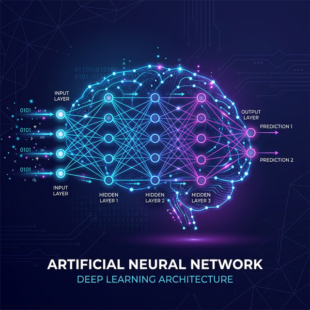
A single perceptron isn't very smart. But when you connect thousands of them together, you create a sprawling "Neural Network". A standard ann deep learning architecture is divided into three distinct vertical stages:

• Input Layer: The very first wall of neurons. It receives the raw data (like the pixels of an image or columns in a spreadsheet) and passes it inside.
• Hidden Layers: This is where the "Deep" in Deep Learning comes from! The hidden layers neural network architecture consists of multiple dense columns of neurons. They perform complex mathematical transformations to extract hidden features (like recognizing the curve of a cat's ear).
• Output Layer: The final wall of neurons that spits out the final prediction (e.g., predicting 95% probability the image is a 'Cat').

3. Activation Functions (The Brain's Mathematical Filters)

If a neural network only multiplied weights and added biases, it would essentially just be a giant, linear math equation. It could never solve complex, curvy, non-linear real-world problems. This is where activation functions relu sigmoid and others step in.

• ReLU (Rectified Linear Unit): The most popular activation function for hidden layers. If a neuron calculates a negative number, ReLU turns it to 0 (turns the neuron off). If it is positive, it lets the number pass through. It is incredibly fast and avoids the vanishing gradient problem.
• Sigmoid: Primarily used in the final Output Layer for binary classification. It mathematically squishes any number into a probability perfectly bounded between 0 and 1.
• Softmax: Used exclusively in the final Output Layer for multi-class classification (e.g., predicting between Cat, Dog, or Bird) making sure all output probabilities perfectly add up to 100%.

4. How the Network "Learns": Backpropagation

When you first create a network, the mathematical weights connecting the neurons are completely randomized. Its first few predictions will be hilariously wrong. How does it learn?

Through the legendary backpropagation algorithm (Backward Propagation of Errors). The network checks its prediction against the actual answer key and calculates how overwhelmingly "wrong" it was (using a Loss Function). It then hits reverse, traveling backward through the entire network, adjusting and fine-tuning every single weight using calculus (Gradient Descent) so it is slightly less wrong the next time. It repeats this forward-backward loop millions of times.

5. Practical Python Implementation (TensorFlow / Keras)

In the modern era, you do not need to write the complex calculus from scratch. Here is standard neural network python code keras to build a functional Artificial Neural Network used to predict customer churn (binary classification) using TensorFlow and Keras.

# 1. Import TensorFlow and Keras Sequential Model
import numpy as np
import tensorflow as tf
from tensorflow.keras.models import Sequential
from tensorflow.keras.layers import Dense
from sklearn.model_selection import train_test_split
from sklearn.preprocessing import StandardScaler

# 2. Simulated Customer Data (Age, Account Balance, Credit Score) -> Churned (1 or 0)
X = np.array([[25, 4000, 600], [50, 85000, 800], [35, 200, 500], [45, 120000, 750], [22, 100, 550]])
y = np.array([1, 0, 1, 0, 1])

# 3. Train/Test Split and Feature Scaling (CRITICAL FOR NEURAL NETWORKS)
X_train, X_test, y_train, y_test = train_test_split(X, y, test_size=0.2, random_state=42)
scaler = StandardScaler()
X_train_scaled = scaler.fit_transform(X_train)

# 4. Build the ANN Architecture
model = Sequential()

# Input Layer & First Hidden Layer (3 Input Features, 8 Neurons, ReLU Activation)
model.add(Dense(units=8, activation='relu', input_shape=(3,)))

# Second Hidden Layer (4 Neurons)
model.add(Dense(units=4, activation='relu'))

# Output Layer (1 Neuron, Sigmoid Activation for Binary Probability 0 to 1)
model.add(Dense(units=1, activation='sigmoid'))

# 5. Compile the Model (Attach the Optimizer and Cost Function)
model.compile(optimizer='adam', loss='binary_crossentropy', metrics=['accuracy'])

# 6. Train the Neural Network via Backpropagation! (epochs = number of loops)
model.fit(X_train_scaled, y_train, batch_size=2, epochs=50)

Conclusion

The dawn of deep learning basics has forever shifted the paradigm of artificial intelligence. While traditional machine learning hits a ceiling regarding how much data it can absorb, Artificial Neural Networks actually scale infinitely in power; the more data you feed them, the smarter they become. However, they demand massive amounts of computational GPU power and incredibly large, clean datasets to achieve their maximum potential.