K-Nearest Neighbors (KNN) Algorithm: Complete Guide

Welcome to this intuitive guide exploring the knn algorithm machine learning methodology. Often described as the most accessible algorithm for beginners, K-Nearest Neighbors elegantly solves complex problems using arguably the simplest rule of life: "Tell me who your friends are, and I'll tell you who you are."

1. What is the K-Nearest Neighbors Algorithm?

A comprehensive k-nearest neighbors explanation begins with its core definition. KNN is a supervised learning algorithm heavily utilized for both classification and regression tasks. However, unlike robust models like Decision Trees or Logistic Regression, KNN completely bypasses building a mathematical equation or complex "model structure" in the background.

Instead, it acts as a "Lazy Learner". It simply memorizes the entire dataset during training. When you introduce a brand new, unknown data point, the algorithm measures how physically close it is to the existing points (neighbors) on the graph. It counts the votes of the 'K' closest neighbors to decide the new point's classification.

2. KNN Distance Metrics: The Math Behind the Magic

How does the machine mathematically calculate "closeness"? It utilizes structured knn distance metrics. Depending on the dimensionality and type of numeric data, KNN can apply several different geometric calculations:

Euclidean Distance: The most common metric. It calculates the straight, direct line distance between two points (analogous to the Pythagorean theorem). Best used for continuous real-world numerical data.
Manhattan Distance: Also known as city-block distance. It strictly calculates distance by navigating along grid lines at 90-degree angles (like walking around city blocks). Very useful for high-dimensional data.
Minkowski Distance: A generalized mathematical formula that technically encompasses both Euclidean and Manhattan depending on a tuned parameter 'p'.

3. How to Choose 'K' in KNN?

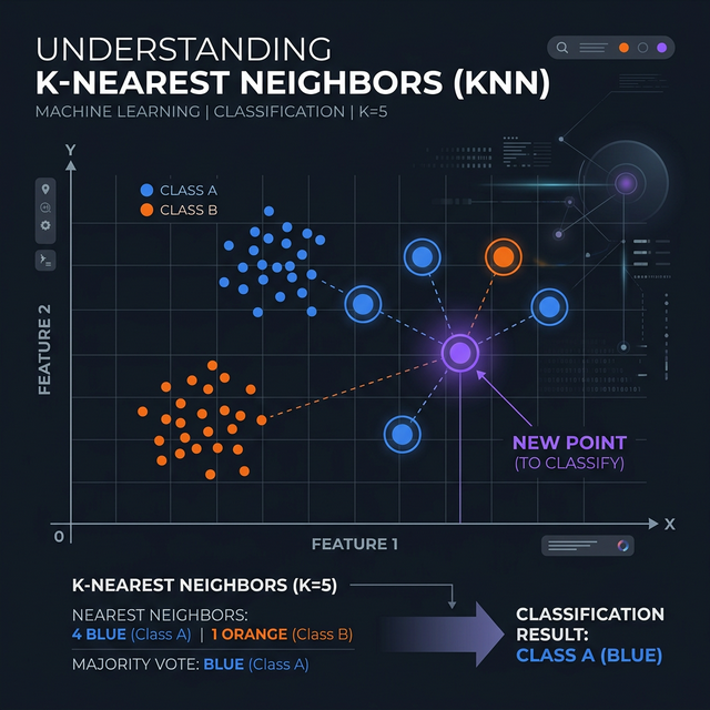
The "K" in KNN literally represents the number of neighbors the algorithm checks before making a decision. Knowing how to choose k in knn is the primary tuning job of a data scientist.

If you set K = 1, the new data point simply copies the exact identity of whatever single point happens to be closest. This creates highly jagged boundaries and extreme overfitting. However, if you set K = 100 on a dataset of 150 points, it will massively "underfit", almost always voting for whatever majority class dominates the entire dataset regardless of local proximity.

Rule of Thumb: Typically, you calculate the square root of the total number of data points (N) in your dataset to find a solid baseline K. Furthermore, if you are attempting a binary classification (e.g., Cat or Dog), always ensure 'K' is an odd number (3, 5, 7) to completely prevent tie-breaker null votes!

4. Practical KNN Python Code Implementation

Deploying this logic natively in Python is blissfully simple. Below is standardized knn python code utilizing the highly respected scikit-learn library documentation. In this example, we predict a user's likelihood to purchase a car based on Age and Estimated Salary.

Crucial Note: Because KNN relies strictly on geometric mathematical distances, you must scale/normalize your data first, otherwise the "Salary" column (measured in thousands) will completely overshadow the "Age" column (measured in tens).

# 1. Import necessary components
import numpy as np
import pandas as pd
from sklearn.model_selection import train_test_split
from sklearn.preprocessing import StandardScaler
from sklearn.neighbors import KNeighborsClassifier
from sklearn.metrics import accuracy_score, confusion_matrix

# 2. Simulated Dataset: [Age, Salary] -> Bought Car? 1(Yes) or 0(No)
X = np.array([[22, 25000], [25, 30000], [47, 85000], [52, 105000], [46, 50000], [35, 65000], [19, 15000], [60, 150000]])
y = np.array([0, 0, 1, 1, 1, 0, 0, 1])

# 3. Train-Test Split 
X_train, X_test, y_train, y_test = train_test_split(X, y, test_size=0.25, random_state=42)

# 4. Feature Scaling (REQUIRED FOR KNN)
scaler = StandardScaler()
X_train_scaled = scaler.fit_transform(X_train)
X_test_scaled = scaler.transform(X_test)

# 5. Initialize KNN (Using n_neighbors = 3, Euclidean metric = minkowski with p=2)
knn = KNeighborsClassifier(n_neighbors=3, metric='minkowski', p=2)

# 6. Fit the model to scaled training data
knn.fit(X_train_scaled, y_train)

# 7. Predict & Evaluate
predictions = knn.predict(X_test_scaled)

print(f"KNN Accuracy: {accuracy_score(y_test, predictions) * 100}%")
print("\nConfusion Matrix:\n", confusion_matrix(y_test, predictions))

Conclusion

The **KNN algorithm in machine learning** is a spectacular introduction to data-driven AI inference. While it might noticeably slow down and suffer from "The Curse of Dimensionality" on absolutely massive datasets (because it has to calculate the distance to *every single point* in existence during the prediction phase), it remains highly accurate, perfectly interpretable, and wildly successful for small-to-mid scale analytics.

Frequently Asked Questions (FAQs)

Why is KNN called a "lazy" algorithm?

Unlike neural networks or logistic regression that spend hours "training" an optimized mathematical weight equation in the background, KNN skips training entirely. It just stores the raw data in RAM. It only "wakes up" and runs aggressive calculations at the exact moment you ask it to make a prediction on a new point, meaning prediction times are incredibly slow compared to other models.

What is "The Curse of Dimensionality" in KNN?

KNN functions beautifully inside 2D, 3D, and 4D feature spaces. However, if your dataset has 1,000 different features (dimensions), the mathematical distance between standard data points mathematically converges toward a similar average. The concept of "closeness" practically loses its definition in extremely high dimensions, crippling the reliability of KNN.

Can KNN perform Regression (predicting a number instead of a class)?